Purchase your New Stata 19 Student License here, with rapid downloads sent directly to your inbox.
Complete Your Order Here
Choose the number of licenses, license term and the product you are after and add to basket.
Navigate to 'compare versions' below to discover more about each flavour of Stata. Still need help? Contact us to discuss your requirements.
Navigate here to purchase, lab licenses start at 10 users.
Comparer Stata
Stata est une suite logicielle complète et intégrée qui répond à tous vos besoins en science des données : manipulation, visualisation, statistiques et reporting automatisé. Stata n'est pas vendu sous forme de modules, ce qui signifie que vous disposez de tout ce dont vous avez besoin dans une seule et même solution.
Que vous soyez étudiant ou professionnel de la recherche chevronné, une gamme de packages Stata est disponible et conçue pour répondre à tous les besoins.
Toutes les éditions suivantes de Stata disposent du même ensemble complet de commandes et de fonctionnalités, ainsi que de manuels inclus sous forme de documentation PDF dans Stata.

Stata/MP est l'édition la plus rapide et la plus complète de Stata. Pratiquement tous les ordinateurs actuels peuvent bénéficier du multitraitement avancé de Stata/MP. Cela inclut les processeurs Intel i3, i5, i7, i9, Xeon et Celeron, ainsi que les puces multicœurs AMD. Sur les puces double cœur, Stata/MP est globalement 40 % plus rapide et 72 % plus rapide là où c'est nécessaire, sur les commandes d'estimation chronophages. Avec plus de deux cœurs ou processeurs, Stata/MP est encore plus rapide.
Stata/MP est plus rapide, bien plus rapide. Stata/MP vous permet d'analyser vos données deux fois plus vite, voire deux fois plus vite que Stata/SE sur les ordinateurs portables bicœurs bon marché, et quatre fois plus vite, voire deux fois plus vite, sur les ordinateurs portables et de bureau quaternaires.
Stata/MP est encore plus rapide sur les serveurs multiprocesseurs. Stata/MP prend en charge jusqu'à 64 processeurs/cœurs.
La vitesse est souvent un critère crucial lors de l'exécution de procédures d'estimation exigeantes en calculs. Certaines procédures d'estimation de Stata, notamment la régression linéaire, sont presque parfaitement parallélisées : elles s'exécutent deux fois plus vite sur deux cœurs, quatre fois plus vite sur quatre cœurs, huit fois plus vite sur huit cœurs, etc. Certaines commandes d'estimation sont plus parallélisables que d'autres. En moyenne, les commandes d'estimation s'exécutent 1,8 fois plus vite sur deux cœurs, 2,9 fois plus vite sur quatre cœurs et 4,1 fois plus vite sur huit cœurs.
Stata/MP est entièrement compatible avec les autres éditions de Stata. Les analyses n'ont pas besoin d'être reformulées ou modifiées pour bénéficier des améliorations de vitesse de Stata/MP.
Stata/MP est disponible pour les systèmes d'exploitation suivants :
- Windows (processeurs 64 bits) ;
- macOS (processeurs Intel 64 bits) ;
- Linux (processeurs 64 bits) ;
Pour exécuter Stata/MP, vous pouvez utiliser un ordinateur de bureau équipé d'un processeur double ou quadruple cœur, ou un serveur multiprocesseur. Qu'un ordinateur soit équipé de processeurs distincts ou d'un processeur multicœur n'a aucune importance. Plus il y a de processeurs ou de cœurs, plus Stata/MP est rapide.
Pour plus de conseils sur l'achat/la mise à niveau vers Stata/MP ou pour des questions sur le matériel, veuillez contacter notre équipe commerciale.

Stata/SE et Stata/BE ne diffèrent que par la taille de l'ensemble de données qu'ils peuvent analyser. Stata/SE et Stata/MP peuvent ajuster des modèles avec davantage de variables indépendantes que Stata/BE (jusqu'à 65 532). Stata/SE peut analyser jusqu'à 2 milliards d'observations.

Stata/BE autorise des jeux de données contenant jusqu'à 2 048 variables. Le nombre maximal d'observations est de 2,14 milliards. Stata/BE peut contenir jusqu'à 798 variables indépendantes dans un modèle.
| Product Features | Stata/BE | Stata/SE | Stata/MP |
|---|---|---|---|
|
Maximum number of variables Up to 2,048 Variables Up to 32,767 variables Up to 120,000 variables |
|
|
|
|
Maximum number of observations Up to 2.14 billion Up to 20 billion |
|
|
|
|
Speed Comparisons Fast Twice as fast
|
|
|
|
|
Time to run logistic regression with 10 million observations and 20 covariates 20 seconds 10 seconds |
|
|
|
|
Complete suite of statistical features |
 |
 |
|
|
Publication-quality graphics |
|
|
|
|
Extensive data management facilities |
|
|
|
|
Truly reproducible research |
|
|
|
|
Comprehensive reporting and table generation |
|
|
|
|
Powerful programming language |
|
|
|
|
Complete PDF documentation |
|
|
|
|
Exceptional technical support |
|
|
|
|
Includes within-release updates through StataNow |
|
|
|
|
Windows, macOS and Linux |
|
|
|
|
And much more for all your data science needs |
|
|
|
|
Memory requirements |
1GB | 2GB | 4GB |
|
Disk space requirements |
2GB | 2GB | 2GB |
Quoi de neuf dans Stata 19
Approfondissez vos recherches avec les dernières fonctionnalités de Stata 19.
Stata 19 a quelque chose à offrir à chacun. Nous présentons ci-dessous les points forts de cette version. Stata 19 est unique car la plupart des nouvelles fonctionnalités sont accessibles aux chercheurs de toutes disciplines.
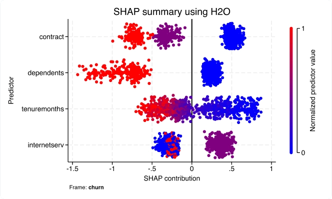
Apprentissage automatique via H2O : arbres de décision d'ensemble
Avec la nouvelle suite h2oml, utilisez le machine learning via H2O pour extraire des informations pertinentes de vos données lorsque les modèles statistiques traditionnels sont insuffisants. Les méthodes de machine learning sont souvent utilisées pour résoudre des problèmes de recherche et d'entreprise axés sur la prédiction.
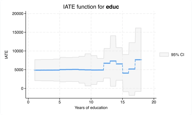
Effets moyens conditionnels du traitement (CATE)
Avec la nouvelle commande cate, vous pouvez aller au-delà de l’estimation d’un effet de traitement global pour estimer des effets individualisés ou spécifiques à un groupe qui répondent à ces types de questions de recherche.
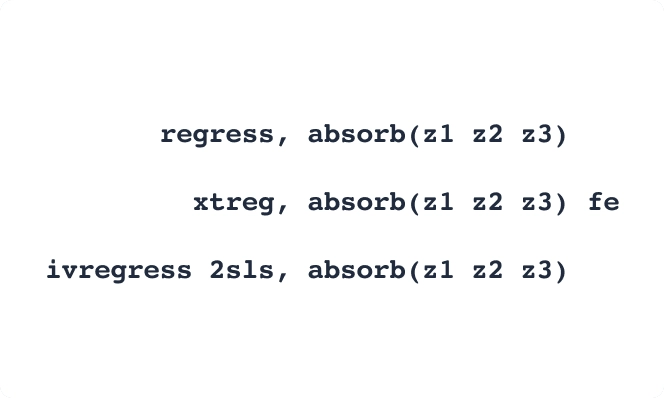
Effets fixes haute dimension (HDFE)
Absorbez non pas une mais plusieurs variables catégorielles de grande dimension dans vos modèles linéaires et à effets fixes avec l'option absorb() des commandes areg et xtreg.
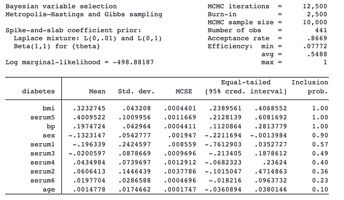
Sélection de variables bayésiennes pour la régression linéaire
Grâce à la nouvelle commande bayesselect, vous pouvez effectuer une sélection bayésienne de variables pour la régression linéaire. Cette approche offre une interprétation intuitive et une inférence stable, tenant compte de l'incertitude du modèle.
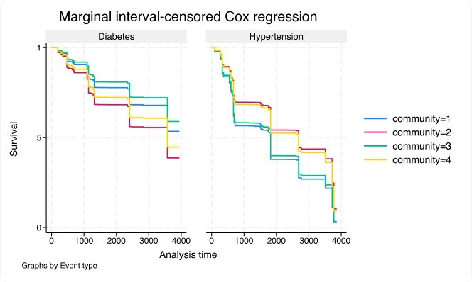
Modèles marginaux de Cox PH pour les données d'événements multiples censurées par intervalle
Utilisez la nouvelle commande stmgintcox pour analyser les données d’événements multiples censurées par intervalle.
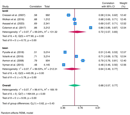
Méta-analyse des corrélations
La suite méta prend désormais en charge la méta-analyse (MA) d'un coefficient de corrélation. Toutes les fonctionnalités standard de méta-analyse, telles que les graphiques en forêt et l'analyse de sous-groupes, sont prises en charge.
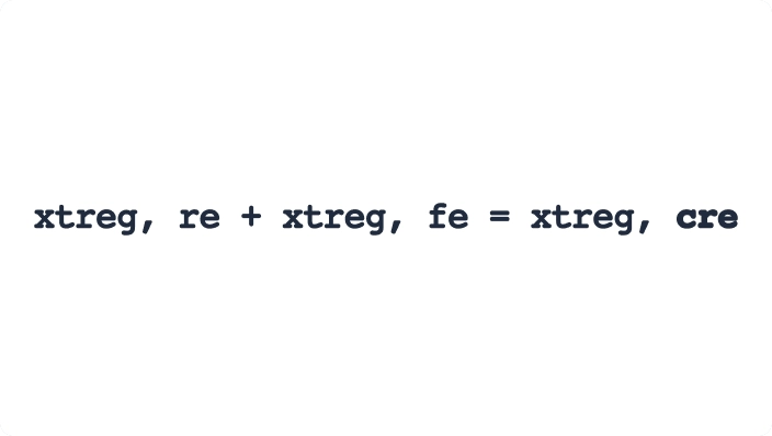
Modèle à effets aléatoires corrélés (CRE)
Vous souhaitez estimer les coefficients des covariables invariantes dans le temps dans votre modèle de données de panel ? Avec xtreg, cre , vous pouvez désormais ajuster un modèle à effets aléatoires corrélés.
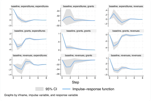
Modèle vectoriel autorégressif (VAR) basé sur des données de panel
Avec la nouvelle commande xtvar, vous pouvez désormais ajuster un modèle vectoriel autorégressif (VAR) de données de panel pour analyser les trajectoires de variables associées lorsque vous observez plusieurs unités ou panneaux au fil du temps.
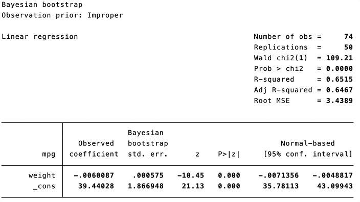
Bootstrap bayésien et pondérations répliquées
Vous pouvez utiliser le nouveau préfixe bayesboot pour effectuer un bootstrap bayésien des statistiques produites par les commandes officielles et celles de la communauté. Le bootstrap bayésien peut intégrer des informations a priori pour obtenir des estimations de paramètres plus précises.
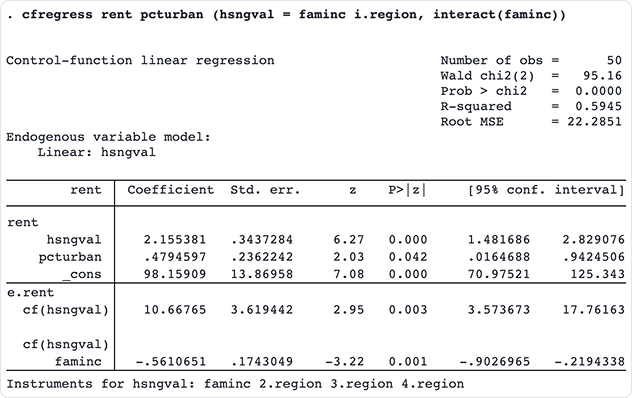
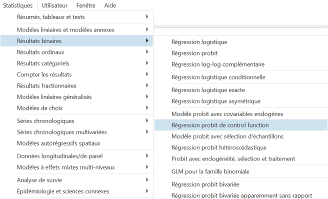
Modèles linéaires et probit à fonction de contrôle
Ajustez les modèles linéaires et probits à fonction de contrôle avec les nouvelles commandes cfregress et cfprobit. Les modèles à fonction de contrôle offrent une approche plus flexible que les méthodes traditionnelles à variables instrumentales (VI) en incluant des variables endogènes.
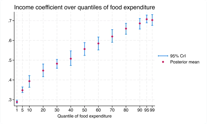
Régression quantile bayésienne via la vraisemblance asymétrique de Laplace
La nouvelle commande bayes:qreg s'adapte à la régression quantile bayésienne. Le cadre bayésien fournit des distributions postérieures complètes pour les coefficients de régression quantile, offrant ainsi une inférence complète.
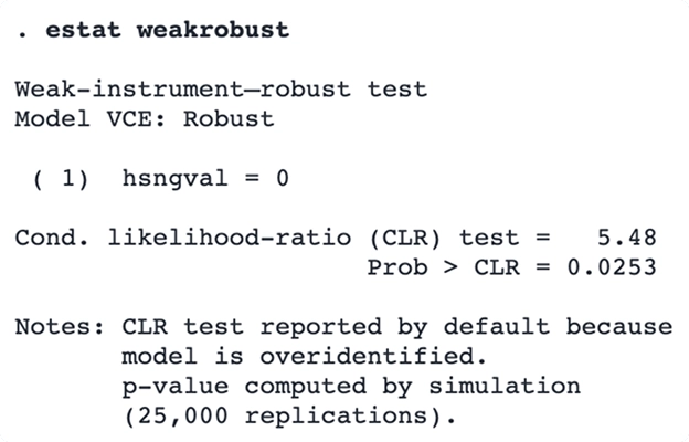
Inférence robuste aux instruments faibles
Utilisez la nouvelle commande estat weakrobust pour effectuer une inférence fiable sur les régresseurs endogènes.
Modèles vectoriels autorégressifs structurels (SVAR) via des variables instrumentales
Avec la nouvelle commande ivsvar, vous pouvez utiliser des instruments au lieu de contraintes à court terme pour estimer les effets causaux dynamiques.
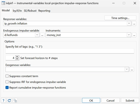
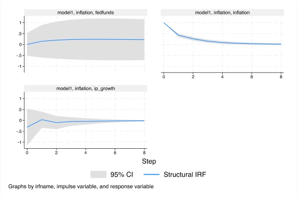
FRI à projection locale à variables instrumentales
Avec la nouvelle commande ivlpirf, vous pouvez prendre en compte l’endogénéité lors de l’utilisation de projections locales pour estimer les effets causaux dynamiques.
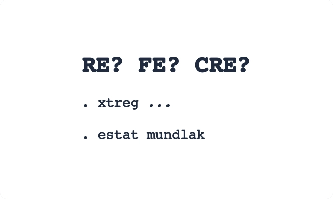
Test de spécification Mundlak
Utilisez la nouvelle commande de post-estimation estat mundlak après xtreg pour choisir entre des modèles à effets aléatoires (RE), à effets fixes (FE) ou à effets aléatoires corrélés (CRE), même avec des erreurs standard robustes en cluster, bootstrap ou jackknife.
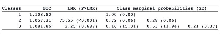
Statistiques de comparaison de modèles de classes latentes
Avec la nouvelle commande lcstats n, vous pouvez utiliser des statistiques telles que l'entropie et une variété de critères d'information pour vous aider à déterminer le nombre approprié de classes.
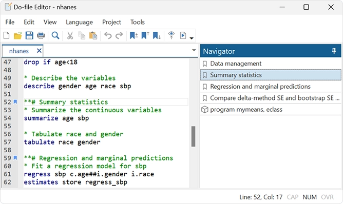
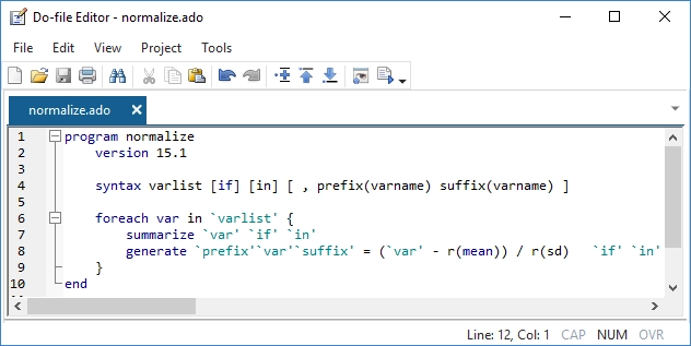
Éditeur Do-file : saisie semi-automatique, modèles et plus encore
L'éditeur Do-file présente les ajouts suivants : saisie semi-automatique des noms de variables, des macros et des résultats stockés ; améliorations du pliage de code ; signets temporaires et permanents ; modèles, onglets et panneau de navigation.
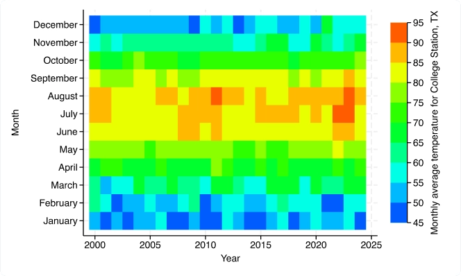
Graphiques : graphiques à barres CI, cartes thermiques et plus encore
Nouvelles fonctionnalités graphiques : Cartes thermiques (bidirectionnelles) ; Tracé de plage et de points avec pics plafonnés (bidirectionnelles) ; Tracé de plage et de points avec pics (bidirectionnelles) ; Étiquetage amélioré, CI et contrôle des regroupements pour les graphiques à barres, les graphiques à points et les boîtes à moustaches ; Couleurs par variable pour plus de graphiques.
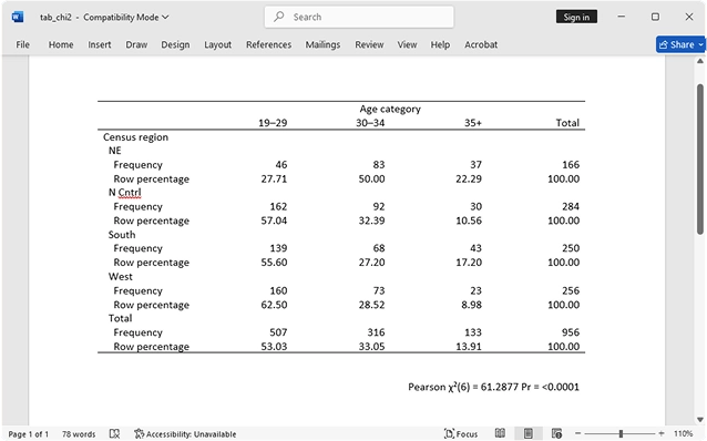
Tableaux : tabulations, exportations et bien plus encore plus faciles
Créez et personnalisez facilement des tableaux avec des titres, des notes et des exportations. La commande « tableau » est un outil flexible permettant de créer des tabulations, des tableaux de statistiques récapitulatives, des tableaux de résultats de régression, etc.
Stata en français
Les menus, boîtes de dialogue et autres éléments de Stata peuvent désormais être affichés en français. Si la langue de votre ordinateur est définie sur le français (fr), Stata utilisera automatiquement le paramètre français.
System Requirements
| OS | Windows 10 Macs avec Apple Silicon et macOS 10.13 ou plus récent pour Macs avec processeurs Intel |
|---|---|
| Processor | Processeur Apple Silicon, Intel ou AMD (Core i3 ou plus) |
| Memory | Stata/MP > 4GB, Stata/SE > 2GB, and Stata/BE 1GB |
| Hard Drive | 4 Go |
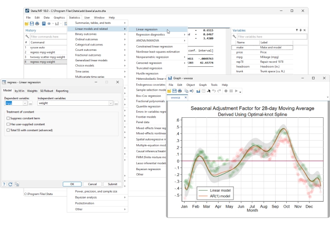
Pourquoi Stata ?
Rapide. Précis. Facile à utiliser. Stata est un logiciel complet et intégré qui répond à tous vos besoins en science des données : manipulation, visualisation, statistiques et reporting automatisé.
|
|
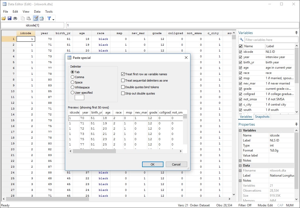
Maîtrisez vos données
Les fonctionnalités de gestion des données de Stata vous offrent un contrôle total.
|
|
Graphiques de qualité des publications
Stata facilite la génération de graphiques de qualité publication, au style distinctif.
Vous pouvez pointer et cliquer pour créer un graphique personnalisé. Vous pouvez également écrire des scripts pour générer des centaines, voire des milliers de graphiques.
de manière reproductible.
Exportez des graphiques au format EPS ou TIFF pour publication, au format PNG ou SVG pour le Web ou au format PDF pour visualisation.
Avec l'éditeur de graphiques intégré, vous cliquez pour modifier quoi que ce soit sur votre graphique ou pour ajouter des titres, des notes, des lignes, des flèches et du texte.
Rapports automatisés
Tous les outils dont vous avez besoin pour automatiser le reporting de vos résultats.
- Document Markdown dynamique
- Créer des documents Word
- Créer des documents PDF
- Créer des fichiers Excel
- Tables personnalisables
- Schémas pour les graphiques
- Word, HTML, PDF, SVG, PNG
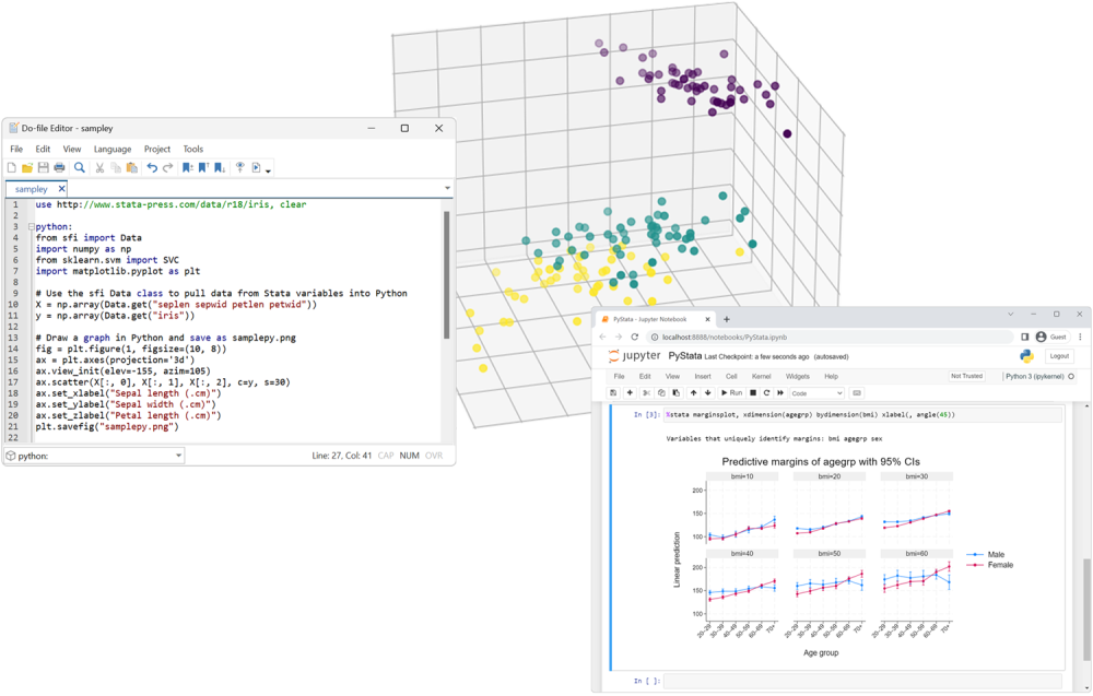
PyStata - Intégration Python
Invoquez Python de manière interactive ou intégrez Python dans votre code Stata.
Appelez Stata depuis Python et appelez le code Stata depuis les environnements IPython.
Utilisez Stata dans Jupyter Notebook.
Transmettez de manière transparente les données et les résultats entre Stata et Python.
Utilisez les analyses Stata depuis Python.
Utilisez n'importe quel package Python dans Stata
- Matplotlib et Seaborn pour la visualisation
- Belle soupe et Scrapy pour le web scraping
- NumPy et pandas pour l'analyse numérique
- TensorFlow et scikit-learn pour l'apprentissage automatique
- Et bien plus encore
Des recherches véritablement reproductibles
On parle beaucoup de recherche reproductible. Stata s'y consacre depuis plus de 30 ans.
Nous ajoutons constamment de nouvelles fonctionnalités ; nous avons même fondamentalement modifié des éléments de langage. Peu importe. Stata est le seul logiciel statistique intégrant le versioning. Si vous avez écrit un script pour effectuer une analyse en 1985, ce même script fonctionnera toujours et produira les mêmes résultats aujourd'hui. Vous pouvez lire tous les jeux de données créés en 1985 aujourd'hui. Et il en sera de même en 2050. Stata pourra exécuter tout ce que vous faites aujourd'hui.
Nous prenons la reproductibilité au sérieux.
Documentation réelle
Lorsqu'il s'agit d'effectuer vos analyses ou de comprendre les méthodes que vous utilisez, Stata ne vous laisse pas tomber et ne vous oblige pas à commander des livres pour apprendre chaque détail.
Chacune de nos fonctionnalités de gestion de données est entièrement expliquée, documentée et illustrée par des exemples concrets. Chaque estimateur est entièrement documenté et inclut plusieurs exemples basés sur des données réelles, accompagnés de discussions concrètes sur l'interprétation des résultats. Ces exemples vous fournissent les données nécessaires pour travailler avec Stata et même étendre vos analyses. Nous vous proposons un guide de démarrage rapide pour chaque fonctionnalité, présentant certaines des utilisations les plus courantes. Besoin de plus de détails ? Nos sections Méthodes et formules détaillent les calculs effectués, et nos références vous orientent vers des informations complémentaires.
Stata est un logiciel volumineux, avec une documentation abondante : plus de 18 000 pages réparties en 35 manuels. Pas d'inquiétude : saisissez « Aide mon sujet » et Stata effectuera une recherche parmi ses mots-clés, ses index et même les logiciels proposés par la communauté pour vous fournir tout ce dont vous avez besoin sur votre sujet. Tout est disponible directement dans Stata.
De confiance
Nous ne nous contentons pas de programmer des méthodes statistiques, nous les validons.
Les résultats obtenus avec un estimateur Stata reposent sur des comparaisons avec d'autres estimateurs, des simulations de Monte-Carlo de cohérence et de couverture, et des tests approfondis effectués par nos statisticiens. Chaque Stata que nous livrons a passé avec succès une suite de certification comprenant 4,1 millions de lignes de code de test produisant 5,8 millions de lignes de sortie. Nous certifions chaque chiffre et chaque extrait de texte de ces 5,8 millions de lignes de sortie.
Fiable
Depuis plus de 35 ans, StataCorp est fidèle à ses utilisateurs en enrichissant le logiciel Stata de nouvelles méthodes statistiques et des technologies de pointe en matière de reporting, de visualisation et de manipulation de données, ainsi que d'interface utilisateur. Forts de notre longue expérience en matière de versions, nous nous engageons à fournir en permanence des logiciels stables et fiables à notre communauté diversifiée de chercheurs et de praticiens.
Mise à jour continue
Rester sur la version la plus récente de Stata est désormais plus facile que jamais.
StataCorp développe continuellement de nouvelles fonctionnalités pour améliorer le logiciel Stata, des méthodes statistiques les plus récentes aux meilleurs outils de reporting, de visualisation de données et d'interface utilisateur. Avec StataNow™, de nouvelles fonctionnalités sont déployées tout au long de la version actuelle jusqu'à la prochaine version majeure. Ces fonctionnalités sont priorisées dans le cycle de développement afin d'être disponibles dès leur disponibilité et d'être immédiatement utilisables par les utilisateurs.
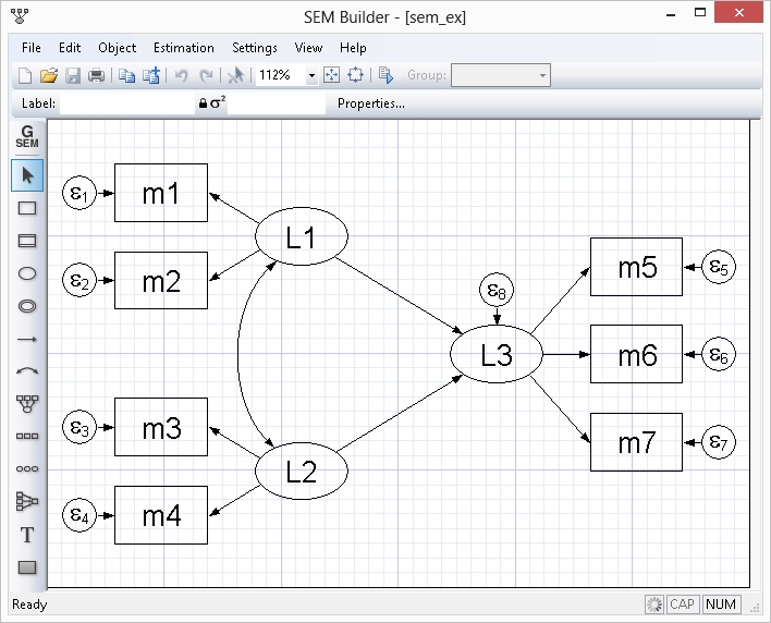
Facile à utiliser
Rester sur la version la plus récente de Stata est désormais plus facile que jamais.
Toutes les fonctionnalités de Stata sont accessibles via des menus, des boîtes de dialogue, des panneaux de configuration, un éditeur de données, un gestionnaire de variables, un éditeur de graphiques et même un générateur de diagrammes SEM. Vous pouvez naviguer dans n'importe quelle analyse en un clic.
Si vous ne souhaitez pas écrire de commandes et de scripts, vous n'êtes pas obligé de le faire.
Même en pointant et en cliquant, vous pouvez enregistrer tous vos résultats et les inclure ultérieurement dans des rapports. Vous pouvez même sauvegarder les commandes créées par vos actions et reproduire ultérieurement votre analyse complète.
Facile à cultiver avec
Les commandes Stata pour l'exécution des tâches sont intuitives et faciles à prendre en main. Mieux encore, tout ce que vous apprenez sur l'exécution d'une tâche peut être appliqué à d'autres tâches. Par exemple, ajoutez simplement « if gender=="female" » à n'importe quelle commande pour limiter votre analyse aux femmes de votre échantillon. Ajoutez simplement « vce(robust) » à n'importe quel estimateur pour obtenir des erreurs types et des tests d'hypothèses robustes à de nombreuses hypothèses courantes.
La cohérence est encore plus poussée. Ce que vous apprenez sur les commandes de gestion des données s'applique souvent aux commandes d'estimation, et inversement. Il existe également une suite complète de commandes de post-estimation permettant d'effectuer des tests d'hypothèse, de former des combinaisons linéaires et non linéaires, de faire des prédictions, de former des contrastes et même d'effectuer des analyses marginales avec des graphiques d'interaction. Ces commandes fonctionnent de la même manière après pratiquement tous les estimateurs.
Le séquençage des commandes pour lire et nettoyer les données, puis effectuer des tests statistiques et des estimations, et enfin communiquer les résultats, est au cœur d'une recherche reproductible. Stata rend ce processus accessible à tous les chercheurs.
Facile à automatiser
Tout le monde a des tâches à effectuer en permanence : créer un type particulier de variable, produire une table particulière, exécuter une séquence d'étapes statistiques, calculer une RMSE, etc. Les possibilités sont infinies. Stata propose des milliers de procédures intégrées, mais certaines de vos tâches sont relativement uniques ou nécessitent une exécution spécifique.
Si vous avez écrit un script pour effectuer votre tâche sur un ensemble de données donné, il est facile de transformer ce script en quelque chose qui peut être utilisé sur tous vos ensembles de données, sur n'importe quel ensemble de variables et sur n'importe quel ensemble d'observations.
Facile à étendre
Certaines des choses que vous automatisez peuvent être si utiles que vous souhaitez les partager avec vos collègues, voire les rendre accessibles à tous les utilisateurs de Stata. C'est très simple. Avec un peu de code, vous pouvez transformer un script d'automatisation en commande Stata. Une commande prenant en charge les fonctionnalités standard des commandes officielles de Stata. Une commande utilisable de la même manière que les commandes officielles.
Programmation avancée
Stata inclut également un langage de programmation avancé : Mata.
Mata possède les structures, les pointeurs et les classes que vous attendez dans votre langage de programmation et ajoute un support direct pour la programmation matricielle.
Bien que Stata ne nécessite pas de savoir programmer, il est rassurant de savoir qu'un langage de programmation rapide et complet fait partie intégrante de Stata. Mata est à la fois un environnement interactif pour la manipulation de matrices et un environnement de développement complet capable de produire du code compilé et optimisé. Il inclut des fonctionnalités spécifiques pour le traitement des données de panel, effectue des opérations sur des matrices réelles ou complexes, offre une prise en charge complète de la programmation orientée objet et est entièrement intégré à tous les aspects de Stata. Stata offre également une intégration Python complète, vous permettant d'exploiter toute la puissance de Python directement depuis votre code Stata.
Stata dispose également de PyStata, qui fournit une intégration Python complète, vous permettant d'exploiter toute la puissance de Python directement à partir de votre code Stata et d'exploiter toute la puissance de Stata à partir de votre code Python.
Stata vous permet même d'intégrer des plugins C, C++ et Java à vos programmes Stata via une API native pour chaque langage. Vous pouvez même intégrer du code Java directement dans votre code Stata !

Fonctionnalités apportées par la communauté
Stata est tellement programmable que les développeurs et les utilisateurs ajoutent chaque jour de nouvelles fonctionnalités pour répondre aux demandes croissantes des chercheurs d'aujourd'hui.
Grâce aux capacités Internet de Stata, de nouvelles fonctionnalités et des mises à jour officielles peuvent être installées sur Internet en un seul clic.
Support technique de classe mondiale
Tous les utilisateurs enregistrés de la version actuelle de Stata (Stata 18) bénéficient d'une assistance technique gratuite. Si vous n'avez pas enregistré votre exemplaire de Stata, veuillez remplir le formulaire d'inscription en ligne.
Notre équipe dédiée de programmeurs et de statisticiens experts Stata est là pour répondre à vos questions techniques. Des solutions complexes de gestion de données à l'obtention d'un graphique parfait, en passant par l'explication d'une erreur standard robuste et la spécification de votre modèle multiniveau, nous avons les réponses.
Compatible multiplateforme
Stata fonctionne sur Windows, Mac et Linux/Unix ; cependant, nos licences ne sont pas spécifiques à chaque plateforme. Ainsi, si vous possédez un ordinateur portable Mac et un ordinateur de bureau Windows, vous n'avez pas besoin de deux licences distinctes pour utiliser Stata. Vous pouvez installer votre licence Stata sur n'importe quelle plateforme prise en charge. Les jeux de données, programmes et autres données Stata peuvent être partagés entre différentes plateformes sans conversion. Vous pouvez également importer rapidement et facilement des jeux de données depuis d'autres logiciels statistiques, feuilles de calcul et bases de données.
Largement utilisé
Utilisé par les chercheurs depuis plus de 35 ans, Stata fournit tout ce dont vous avez besoin pour la science des données : manipulation de données, visualisation, statistiques et rapports automatisés.
Sélectionnez votre discipline et voyez comment Stata peut travailler pour vous.